Time Series Data Labeling​

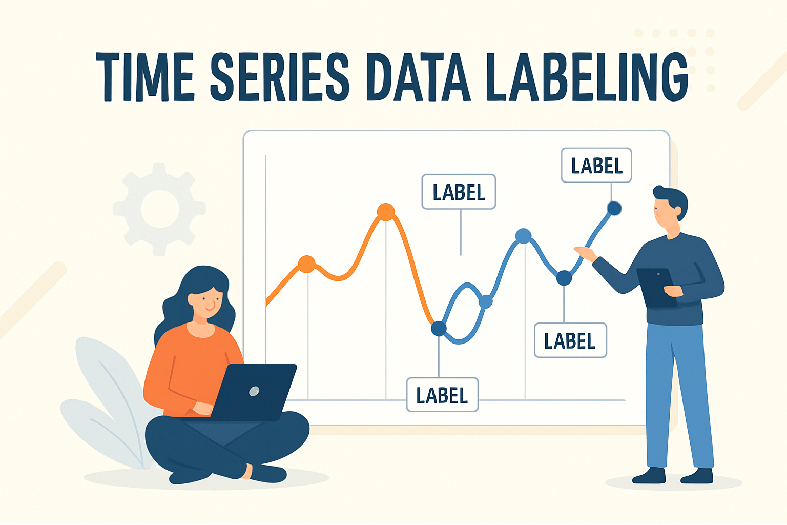
There are several types of machine learning, and one of the most commonly used today is supervised learning. In this category, machine learning models are trained using labeled datasets. The objective of the model is to learn to map the input data to the corresponding labels.

Price series are sequences of prices sampled at fixed intervals, such as every 5 minutes or every day, or based on fixed thresholds, like a certain volume or dollar value. These price series can be labeled to indicate a long, short, or hold action. Technical analysis, for instance, aims to associate past price and volume movements with specific actions, often justified by market psychology. While this article does not evaluate the merits of such an approach, it seeks to make this process more systematic, reducing the need for subjective judgment in each decision using machine learning models.

There are multiple ways to create a model, but the labels typically need to be generated either manually or automatically through some mechanism. Manual labeling has its advantages, such as leveraging the expertise of domain specialists. However, given the vast amount of data available, which can enhance the predictive capabilities of machine learning models, automatic labeling often seems like the most practical solution. The key question, then, is how to approach it. This article explores various automatic labeling methods and compares them by graphing the resulting labels.

Different Approaches in Price Series Labelling

This section will provide a detailed discussion of the different approaches used to label the data. Each subsection will cover the theoretical intuition behind the method, along with the sample illustration of when such labeling method is applied to EUR/USD currency pair for the past two years with one day interval. Following that, the Python implementation will be provided. The interface for each function will be designed to accept a Pandas DataFrame with a column namedClose, along with keyword arguments specific to the implementation. These keyword arguments will have default values to ensure compatibility across different methods. The output of each function will be a pandas DataFrame with three boolean columns: long, short, and hold, which represents the one-hot encoded labels.

Fixed Horizon

The simplest way to label a time series is with a fixed horizon, assigning labels based on price movement within a set window.

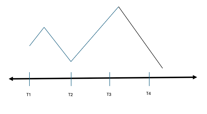
Consider price movement across four intervals, T1 to T4. T2 would be labeled as short if it's lower than T1. A threshold can be applied so that if price movement doesn't reach a specified level, the interval will be labeled hold. The threshold aims to make the labels less susceptible to noice.

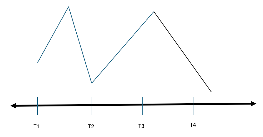
The main drawback of this approach is that it ignores significant price movements between intervals. For example, despite a strong rally between T1 and T2, T2 may still be labeled as short if it's lower than T1. This can lead to triggering stop losses in production, as the approach overlooks such rallies. Additionally, this method assumes that returns are realized exactly within the fixed intervals, which is rarely the case. Predicting both the movement's direction and timing is highly improbable.

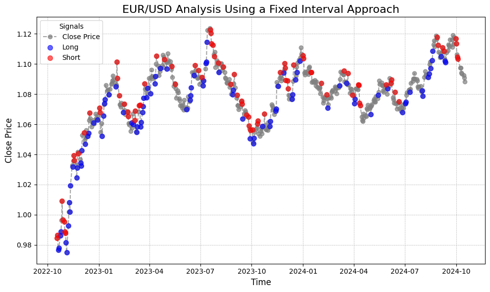
The illustration above showcases the application of this labeling technique on real data, displaying the Euro to USD exchange rate over the past two years. It utilizes a fixed interval of 2 days and a threshold of 0.5% change. The figure highlights a significant drawback of this approach, as it labels intervals are quite unstable, even during times when there is a notable rally on the price.

There are variations of this approach that can address its shortcomings. One method involves considering the high and low prices for each interval to better account for significant price movements between them. Additionally, employing a moving average can help stabilize the price data. However, these methods still have limitations, particularly when applied to datasets with erratic price movements.

Code Implementation

def fixed_interval(data, period=2, min_change=0.005):
  data.loc[:,'buy'] = False
  data.loc[:,'sell'] = False
  data.loc[:,'hold'] = False
  data.loc[:,'future'] = data['Close'].shift(-period)
  data.loc[:,'buy']  = (data['future']  / (data['Close'] ) )-1 > min_change
  data.loc[:,'sell']  = (data['Close'] / (data['future'] ))-1 > min_change
  data.loc[:,'hold']  = data.apply(lambda x: True if x['buy'] == False and x['sell'] ==False else False, axis=1)
  return data

Excess Over Benchmark

Another approach is to label data relative to a benchmark, which could be the mean or median of historical price changes for the asset, market, industry, or a comparable company. This labeling method inherently considers market conditions: bull markets typically exhibit higher overall returns, while the opposite holds true for bear markets.

The effectiveness of this labeling approach hinges on the user's perspective regarding excess returns over the benchmark. Do they believe that any excess return should be compensated by lower future returns, leading the asset to revert to its average? This perspective is often referred to as the mean-reverting view. Conversely, do they interpret excess returns as a sign of market euphoria or confidence in the asset class, allowing them to capitalize on the momentum? This viewpoint is commonly known as the trend-following view.

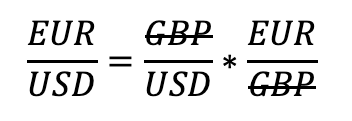
In the context of foreign currency exchange, the relative price change of one currency should align with the relative exchange rate of another currency. This relationship can be illustrated by the equation above. The product of GBP/USD and EUR/GBP cancels the numerator of GBP/USD with the denominator of EUR/GBP, yielding EUR/USD. This reflects a mean-reverting principle, as any discrepancies in these relative exchange rates would typically be arbitraged away in an efficient market. Thus, this approach helps identify such discrepancies, and trading on them contributes to greater market efficiency

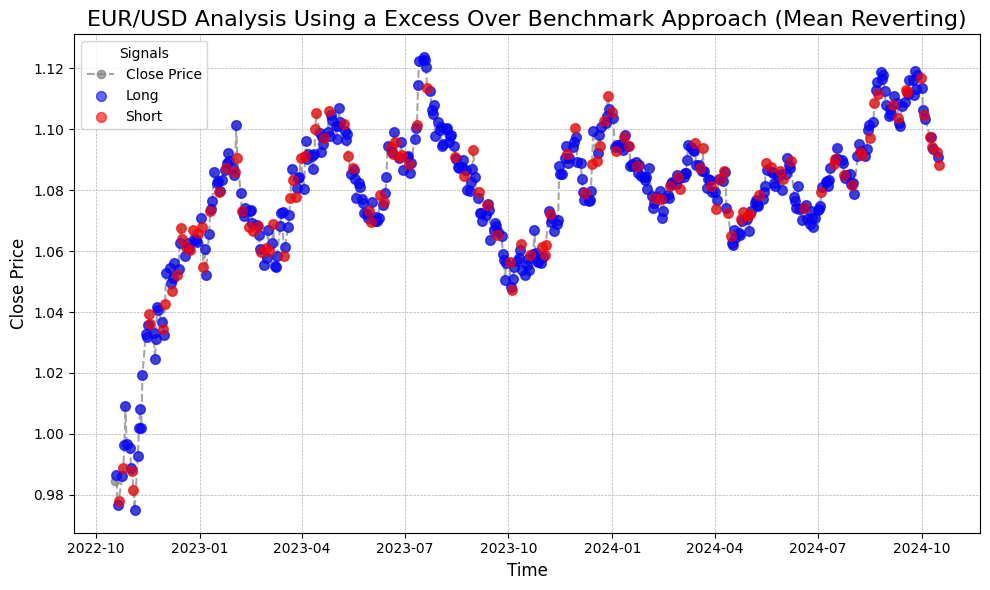
Arbitrage opportunities can persist if the potential profit does not cover the transaction cost. In the graph above, a transaction cost of 0.0001 is assumed. This value represents the minimum difference between the benchmark and the asset class before a long or short label is given. The benchmark is calculated as the price changes of the product of the EUR/GBP and GBP/USD pairs, which is then compared to the price changes of the EUR/USD pair.

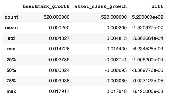
The descriptive statistics for the benchmark growth, asset class growth, and the difference between the asset class and benchmark growth are shown above. The data suggests that EUR/USD tends to decline more often relative to the movement of the two benchmark currency pairs. This is evidenced by the 50% quantile, where the benchmark shows a growth of 0.000024, while EUR/USD exhibits a decline of -0.000093. The mean difference is also negative, though the magnitude is small. This usually requires further analysis to uncover the underlying reasons behind these numbers.

Code Implementation

import pandas as pd
import numpy as np

def excess_over_benchmark_mean_reverting(data, min_change=0.0001):
  data[['buy', 'sell', 'hold']]= False
  data.loc[:, 'growth'] = data['Close'].diff()
  data.loc[:,'buy']  = data['growth'] - data['benchmark']  < min_change
  data.loc[:,'sell']  = data['growth'] - data['benchmark']  > min_change
  data.loc[:,'hold']  = data.apply(lambda x: True if x['buy'] == False and x['sell'] ==False else False, axis=1)
  return data

Expected Return

This labeling approach is inspired by bond valuation methods. Typically, a bond’s price is determined by the present value of all future coupon payments and the principal, discounted at a rate adjusted for risk. In this case, instead of valuing coupon payments, the asset's return is considered, while the principal is the initial cost of entering the position. As long as the expected return exceeds the initial investment, including commission costs, the trade is deemed viable. A fixed window of investment time must be set to implement this although price movements within this fixed window are appropriately considered.

An advantage of this approach is that it discounts distant future returns by the chosen rate, giving more weight to near-term returns while still appropriately accounting for those further in the future.

To implement this method, a fixed investment time window must be established, while still accounting for price movements within this period. The principal value depends on the position taken: for a long position, the principal is a cash outflow at the start of the investment horizon and a cash inflow at the end. Conversely, for a short position, the principal is a cash inflow initially and a cash outflow at the conclusion of the horizon.

To determine the position, the present value of both the long and short positions are compared, and the one with the higher value is selected. If this value exceeds the commission—usually paid upfront, so it doesn't require time value adjustments—then the position will be taken.

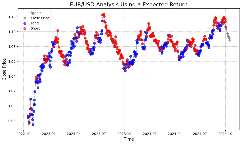
Assuming a commission of 0.00001 and a daily compounded discount rate of 0.026%, which corresponds to 10% annually, with an investment horizon of ten days, the resulting labels are shown above. The labels appear to have accurately captured most of the upward and downward trends, classifying them correctly.

Code Implementation

import pandas as pd
import numpy as np

def expected_return(data, commission=0.00001, discount_rate=0.00026, investment_horizon=10):
  ##only considers gains/loss. not the capital
  data[['buy', 'sell', 'hold']]= False
  indexer = pd.api.indexers.FixedForwardWindowIndexer(window_size=investment_horizon)
  present_values = [1/(1+discount_rate)**(i+1) for i in range(investment_horizon)]
  data.loc[:,'diff']= (data['Close'].diff().fillna(0))
  data.loc[:,'present_value_long'] = data['diff'].rolling(window=indexer, min_periods=investment_horizon).apply(lambda x: sum(x*present_values)) - data['Close'] + (data['Close']/(1+discount_rate)**(investment_horizon))-commission
  data.loc[:,'present_value_short'] = data['diff'].rolling(window=indexer, min_periods=investment_horizon).apply(lambda x: sum(-x*present_values)) + data['Close'] - (data['Close']/(1+discount_rate)**(investment_horizon))-commission
  data.loc[data['present_value_long']>0, 'buy']= True
  data.loc[data['present_value_short']>0, 'sell']= True
  data.loc[:,'hold']  = data.apply(lambda x: False if x['buy'] == True or x['sell'] == True else True, axis=1)
  data[['buy', 'sell', 'hold']] = data[['buy', 'sell', 'hold']].fillna(False)
  return data

Triple Barrier

The book Advances in Financial Machine Learning of Marcos López de Prado proposes a new approach in labeling the numbers that is path dependent and could be adjusted based on the tactical trading requirements such as stop losses and maximum holding period.

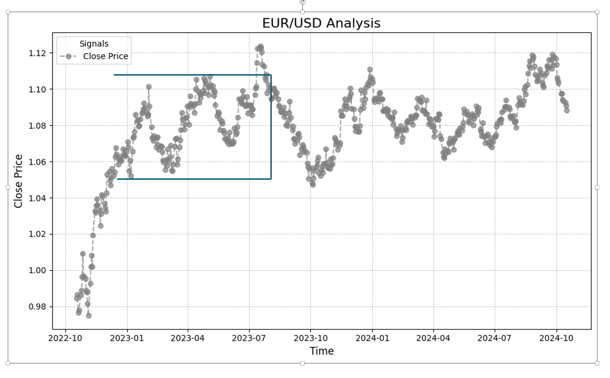
The concept of the triple barrier method involves drawing two horizontal lines and one vertical line. The horizontal lines represent thresholds: when the upper line is reached first, it signals a long position; when the lower line is reached first, it signals a short position. The vertical line represents the maximum holding period, indicating that the trade must be closed if this is reached before either threshold. The horizontal thresholds can be adjusted to set different limits for long and short positions. This labeling technique can also be modified by omitting the vertical barrier, representing the maximum holding period, which is typically a requirement in other methods previously discussed.

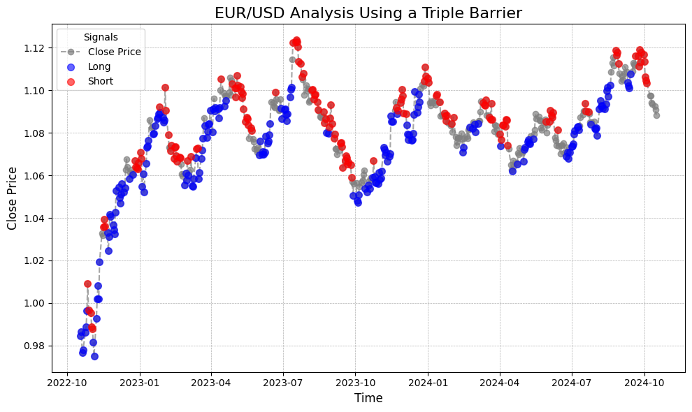
The illustration above depicts how the EUR/USD would be labeled using the Triple Barrier method, a framework designed for effective trading strategies. Utilizing an investment horizon of 10 days with a target gain of 1%, the labels is consistent with the general trend of the prices. Uptrend values, representing bullish momentum, are primarily labeled as long, while downtrend values, indicating bearish momentum, are predominantly labeled as short. This consistency underscores the reliability of the trading signals generated by the Triple Barrier approach, as shown in the visual representation above.

Code Implementation

import pandas as pd
import numpy as np
from numba import jit, prange

## Helper Function
@jit(nopython=True,  cache=True)
def getTripleBarrierLabels(all_prices, max_length, target_gain):
    target_gain_ref = round(target_gain,7)
    transaction_cost=0.00001 #pct
    positions = []
    for i in range(len(all_prices)):
        position=0 #(0 neutral, + buy , - short )
        current_position = all_prices[i] # get the current dataframe
        
        max_range = min(len(all_prices[i:]), max_length+1)
        for j in range(max_range):
            b_current_return = round(all_prices[i+j] / (current_position * (1+transaction_cost)) - 1,7)
            s_current_return = round((current_position * (1-transaction_cost)) / all_prices[i+j] - 1,7)
            if b_current_return>=target_gain_ref:
                position = i+j
                # position = j
                break
            elif s_current_return>=target_gain_ref:
                position = -(i+j)
                # position = -j
                break

        positions.append(position)

    return positions

def triple_barrier(data, investment_horizon=10, target_gain=0.01):
    data.loc[:,'uniqueness_identifier'] =  getTripleBarrierLabels(all_prices= data['Close'].values, max_length=investment_horizon, target_gain=target_gain) #6 hours max holding period
    
    data.loc[:,'buy'] = False
    data.loc[:,'sell'] = False
    data.loc[:,'hold'] = False
    data.loc[:,'hold_period'] = 0

    data['uniqueness_identifier'] = data['uniqueness_identifier'].fillna(0)

    data.loc[data['uniqueness_identifier']>0,'buy'] = True
    data.loc[data['uniqueness_identifier']<0,'sell'] = True
    data.loc[(data['uniqueness_identifier']==0) | (data['uniqueness_identifier'].isna()) ,'hold'] = True


    return data

The approach utilizes a helper function compiled just in time (JIT) to run on machine code using Numba, which significantly speeds up the processing time. This optimized helper function is then employed in the main function to apply the labels efficiently. By leveraging Numba's capabilities, the algorithm enhances performance, enabling quicker and more efficient label generation.

Trend Scanning

Trend Scanning is another novel approach introduced by Marcos López de Prado in his book Machine Learning for Asset Managers. This innovative method simplifies the labeling process by relieving users of the need to set various hyperparameters, such as profit and stop-loss levels and holding periods. Instead, the algorithm focuses on determining the trend direction by fitting multiple regression models along the asset's price path. This dynamic approach eliminates the need for fixed intervals typically required for computing regression lines, allowing for a more accurate representation of market conditions. The algorithm checks, within a specific span, for the slope with the highest t-value. Additionally, a threshold t-value can be set to minimize noise in the labeling process. By applying this threshold, users can filter out less significant trends, ensuring that only statistically robust signals are considered for decision-making.

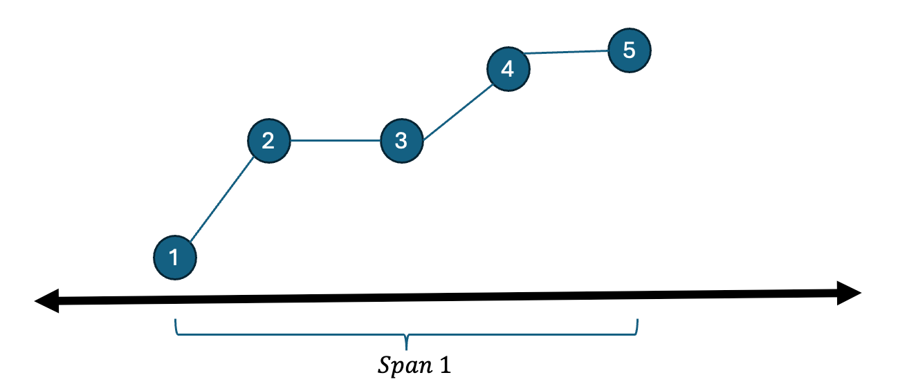
This approach is illustrated above, where a span hyperparameter is set to define the window of analysis. Within this span, a subset of points is checked iteratively by fitting a regression line between point P1 and all subsequent points (e.g., P2​,P3​,P4​,P5​). For each regression line, represented as reg(P1,P2, reg(P1,P3), reg(P1,P4), and reg(P1,P5)reg(P1​,P5​), the t-value is computed. The maximum t-value obtained from these regressions determines the slope that will inform the label for the Trend Scanning method. For instance, if the maximum t-value corresponds to reg(P1,P2) and the slope is positive, the position would be labeled as a long position.

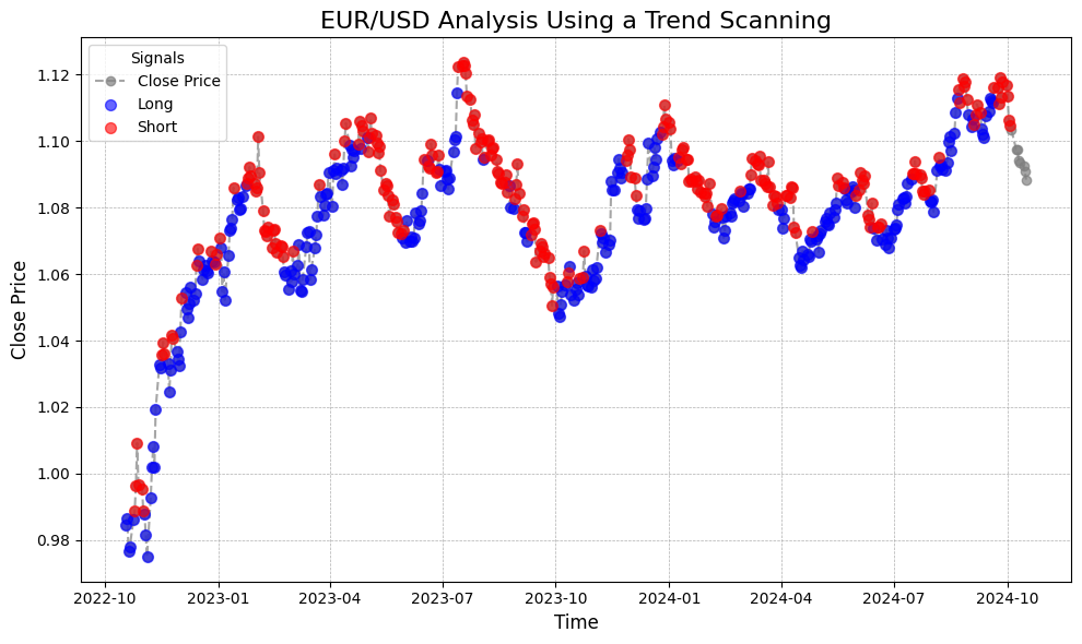
The illustration above demonstrates the Trend Scanning approach applied to the EUR/USD with a span horizon of 10 and a threshold of 0.0001. This method effectively identified most points as long positions during upward trends and classified them as short positions during downward trends. A notable distinction is that the Trend Scanning approach labeled significantly more long and short positions compared to the Triple Barrier Approach, which tends to leave positions in a holding state more often. This increased labeling frequency can provide traders with more opportunities to capitalize on market movements.

Code Implementation

import pandas as pd
import numpy as np
from numba import jit, prange

## Helper function
@jit(nopython=True, cache=True)
def ols_regression(y, X):
    n, k = X.shape
    beta = np.linalg.inv(X.T @ X) @ X.T @ y
    e = y - X @ beta
    RSS = np.sum(e**2)
    dof = n - k
    RSE = np.sqrt(RSS / dof)
    cov_beta = np.linalg.inv(X.T @ X) * RSE**2
    se_beta = np.sqrt(np.diag(cov_beta))
    t_values = beta / se_beta

    return beta, se_beta, t_values

@jit(nopython=True, cache=True)
def tValLinR(close):
    n = close.shape[0]
    X = np.column_stack((np.ones(n), np.arange(n)))
    y = close.astype(np.float64)  # Convert to native type for Numba compatibility

    # Perform OLS regression
    beta, se_beta, t_values = ols_regression(y, X)

    return t_values[1]  # Return t-value for the second coefficient (excluding intercept)


@jit(nopython=True, cache=True)
def getBinsFromTrend(close,span,threshold):
    '''
    Derive labels from the sign of t-value of linear trend
    Output includes:
    - t1: End time for the identified trend
    - tVal: t-value associated with the estimated trend coefficient - bin: Sign of the trend
    '''
    max_length = len(close)
    hrzns=prange(*span)
    out= np.zeros(max_length)
    t_values= np.zeros(max_length)
    for idx in prange(max_length):
        if idx+max(hrzns)>max_length:continue
        max_tvalue = -np.inf
        selected_tvalue=0
        for hrzn in hrzns: 
            end_idx = hrzn+idx
            t_value=tValLinR(close[idx:end_idx])
            abs_tvalue =  abs(t_value)
            if np.isinf(t_value) or np.isnan(t_value):
                t_value=0
            max_tvalue = max(abs_tvalue, max_tvalue)
            if max_tvalue ==abs_tvalue and abs_tvalue>=threshold:
                selected_tvalue=end_idx*np.sign(t_value)
        out[idx] = selected_tvalue
        t_values[idx] = t_value
    return out, t_values

# Main function
def trend_scanning(data, span=10, threshold=0.00001):
  if span<=5:
    print('span must be more than 5')
  else:
      span =  (min(span,4),span,1)
      out, t_values = getBinsFromTrend(data['Close'].values, span=span, threshold=threshold)
      data.loc[:, ['uniqueness_identifier', 'tvlues']] = np.column_stack((out, t_values))
      
      data.loc[:,'buy'] = False
      data.loc[:,'sell'] = False
      data.loc[:,'hold'] = False

      data['uniqueness_identifier'] = data['uniqueness_identifier'].fillna(0)

      data.loc[data['uniqueness_identifier']>0,'buy'] = True
      data.loc[data['uniqueness_identifier']<0,'sell'] = True
      data.loc[(data['uniqueness_identifier']==0) | (data['uniqueness_identifier'].isna()) ,'hold'] = True

      return data

The code implementation above employs helper functions that are compiled to machine code, significantly improving processing speed. It iteratively checks the price series over the specified span horizon, allowing the algorithm to analyze trends effectively within the defined timeframe. This iterative approach ensures that each price point is evaluated, facilitating accurate label generation based on market movements.

Closing Remarks

The labeling methods discussed here all needs to be optimize to make the labels less susceptible to noise. A noisy label can hinder mchine leanring models form learning the mapping between the input and output labels. Threshold values and the time horizon are two hyperparameters that could be played around to make the labeling more robust.