Fractional Differencing: A Better Approach in Price Series Transformation

Price information is a very common metric that investors use to make financial decisions. This is no wonder as price information signals to the investing world how buyers and sellers are reacting to certain information about an asset class. A whole host of techniques, more commonly known as technical analysis, are devoted in using price and volume information to interpret market psychology and predict future market movements. Price information are also melded with the financial and other analytical data to make forecasts.

Price in the Context of Machine Learning

The abundance of price data often makes it the starting point for creating machine learning models. One common use of price data in machine learning is generating a price series—a sequence of prices over a given time interval. More advanced applications may utilize volume-based or dollar-based intervals, where a new sample or tick is generated only after reaching a specific volume or dollar threshold.

Statistical learning typically requires data with a stable mean and variance, commonly referred to as a stationary time series. This is essential because the model learns from the underlying data patterns, and if the data is unstable, the model's predictive power will be compromised. At best, the model will perform well only as long as the mean and variance it was trained on remain consistent. This presents a challenge when modeling financial asset prices, which tend to be non-stationary. This is likely why many people consider prices to follow a random walk.

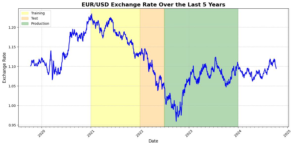
For this demonstration, we will use the exchange rate between the Euro and USD. The dataset consists of daily data from the past five years, sourced from Yahoo Finance. To test the time series for stationarity, we can apply the Dickey-Fuller test, which examines the null hypothesis that a unit root is present in the data. (source: Wikipedia). Unit root is a characteristic of a price series that indicates non-stationarity. This means that the null hypothesis of the Dickey-Fuller test is the price series is non-stationary.

The Augmented Dickey-Fuller (ADF) test statistic for the Euro-USD exchange rate dataset is -1.9070, with a critical value of -3.8370 at the 95% confidence level. Since the test statistic is greater than the critical value (i.e., -1.9070 > -3.8370), we fail to reject the null hypothesis. This indicates that there is insufficient evidence to suggest that the time series is stationary.

To illustrate the issue, consider a scenario where the training data consists solely of the year 2021. This model is then tested on data up to mid-2022 and subsequently deployed in production from mid-2022 to the end of 2023. In this case, the model would likely perform well by predicting a consistently declining exchange rate, as this trend is evident in both the training and testing datasets. However, once deployed, the exchange rate experienced a rally, which could have resulted in significant losses for investors.

Current Approaches on Price Series Transformation

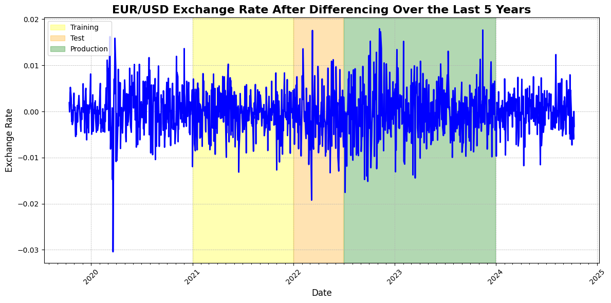
One of the most common methods for transforming a price series into a stationary series is called differencing. Several differencing techniques can be applied to achieve stationarity, including the Random Walk model, second-order differencing, and seasonal differencing. (source: otexts.com). Differencing involves calculating the change between observations, with the reference observation varying depending on the technique. In the Random Walk model, the previous observation is used as the reference point, whereas seasonal differencing takes the observation from the same season as a reference. Second-order differencing applies the Random Walk method twice to the dataset, further stabilizing the time series.

The ADF test statistic for the dataset is -34.9547, with a critical value of -3.8370 at the 95% confidence level. Since the test statistic is less than the critical value (i.e., -34.9547 < -3.8370), we reject the null hypothesis and accept the alternative hypothesis, indicating that the time series is stationary.

The transformation would have rendered the price series suitable for machine learning tasks; however, we are left with a dataset that lacks memory. For instance, around mid-2022, the original dataset would have indicated that the price was at a relatively low point compared to all previous observations, a nuance that is completely lost after the transformation. This information is particularly relevant in the context of foreign currency exchange, as exchange rates typically trade within a narrow band until central banks intervene if fluctuations become excessive. Maintaining this narrow band of exchange values is crucial for ensuring stability in the profitability of companies engaged in foreign transactions and is vital for overall economic growth and stability.

Fractional Differencing

The book Advances in Financial Machine Learning of Marcos López de Prado proposes an alternative method for transforming price series. He argues that differencing does not need to be strictly limited to an integer of 1, as is the case with the random walk transformation. In fact, the book suggests that financial asset price series can be made stationary by applying a differencing value of less than 0.6. For a detailed explanation, I highly recommend reading CHAPTER 5 Fractionally Differentiated Feature of the book.

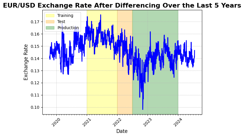
After an iterative search for the optimal value of d—the differencing parameter where d = 1 corresponds to a random walk differencing—the price series was transformed to satisfy the stationarity condition necessary for machine learning, while preserving some price memory. A differencing value ofd = 0.4 successfully transformed the price series into a stationary one. The ADF statistic after fractional differencing is -4.0618, with a critical value of -3.8370 at the 95% confidence level. Since the test statistic is less than the critical value (i.e., -4.0618 < -3.8370), we reject the null hypothesis and accept the alternative hypothesis, indicating that the time series is now stationary. Visual inspection confirms that some price memory remains intact, as the lowest point of the exchange rate is still evident around mid-2022.

Fractional Differencing Implementation

The illustration of the discussion above can be found in the Jupyter Notebook above. The implementation below is adapted from the code suggested in Advances in Financial Machine Learning . A fixed window width is preferred for easier matrix operations in TensorFlow and other deep learning frameworks, as it simplifies the computation and aligns better with the input requirements of these models.

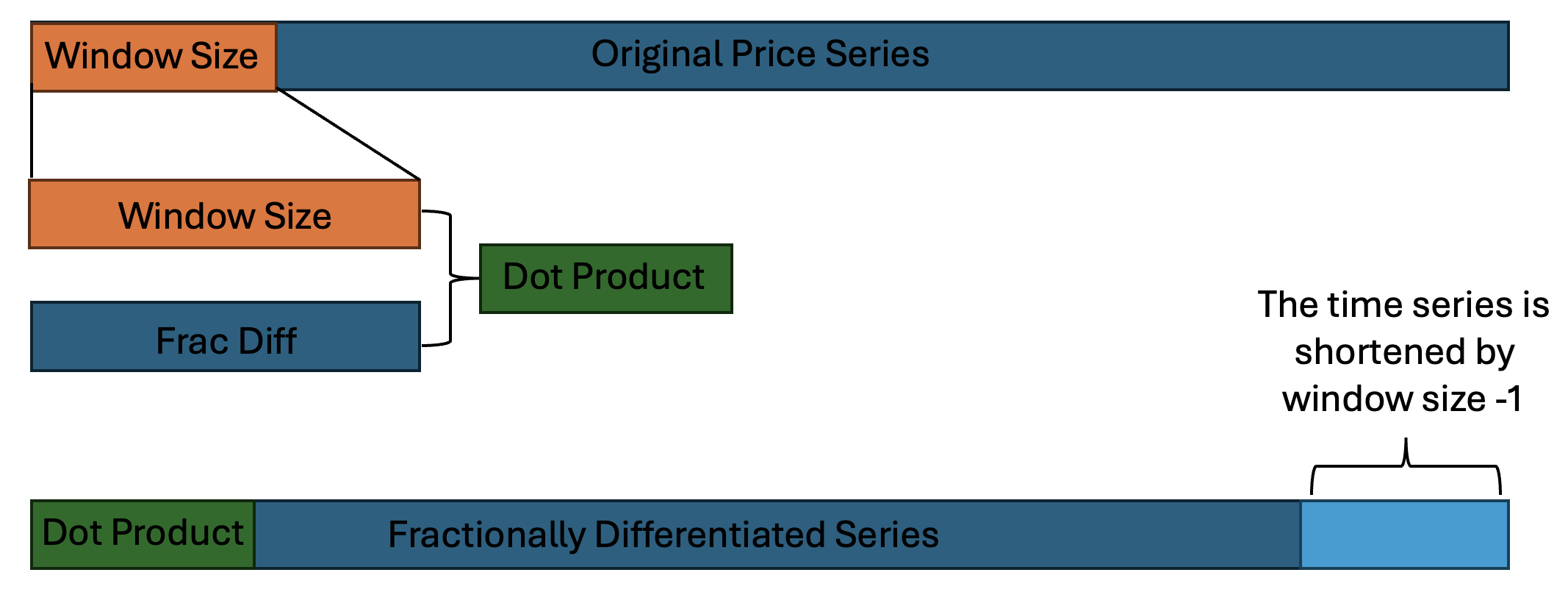
The illustration above demonstrates the general process of transforming the data. A rolling window of size w is applied to the original time series. The dot product between the fixed window and the corresponding fractional differencing weights is computed, forming the first data point in the fractionally differentiated price series. The helper function get_weights_ffd in both the Pandas/Numpy and TensorFlow implementations generates these fractional differencing weights, taking the differencing parameter d and the window size w into account. As a result of this transformation, the output time series will be shorter by w - 1 data points. This must be taken into consideration if this is aligned with non-fractionally differentiated time series, such as macro economic indicators.

The implementation of Fractional Differencing in TensorFlow functions as a preprocessing layer, positioned right after the input layer. The FracDiffLayer allows real-time data transformation before feeding it into the neural network, ensuring that the transformation is bundled with the model itself. The model is initialized with a float value d, which serves as a starting point for differencing. This d is a learnable parameter. Although initial tests show minimal changes in its value, allowing the model to optimize d can improve predictive performance while maintaining stationarity.

Pandas/Numpy Implementation

import numpy as np
import pandas as pd

def fractional_diff_ffd(series, d, window_size):
    """
    Perform fractional differentiation (FFD) on a pandas DataFrame using a sliding window.

    Args:
    - series: A pandas DataFrame with time series data (rows are time steps, columns are features).
    - d: A scalar or array-like fractional differencing order.
    - window_size: The size of the sliding window for FFD.

    Returns:
    - A pandas DataFrame with fractionally differenced data.
    """


    # Helper Function
    def get_weights_ffd(d, window_size):
      w = [1.0]
      k = 1
      for _ in range(window_size - 1):
          w_ = -w[-1] / k * (d - k + 1)
          w.append(w_)
          k += 1
      
      return np.array(w[::-1])

    # Convert series to DataFrame if it's not already
    if isinstance(series, pd.Series):
        series = series.to_frame()
    
    # Ensure d is an array (for compatibility with multi-feature data)
    if not isinstance(d, np.ndarray):
        d = np.array([d] * series.shape[1])
    
    # Calculate the weights for each feature separately
    weights_ffd = np.array([get_weights_ffd(d_i, window_size) for d_i in d])
    
    # Initialize DataFrame for results
    result_df = pd.DataFrame(index=series.index[window_size - 1:], columns=series.columns)
    
    # Apply FFD to each column using the sliding window
    for col_idx, col in enumerate(series.columns):
        series_col = series[col].ffill().dropna()
        frac_diff_col = []

        for i in range(window_size, len(series_col) + 1):
            window_data = series_col.iloc[i - window_size:i].values
            weight = weights_ffd[col_idx]  # Corrected to get the weight for the specific column
            frac_diff_value = np.dot(weight, window_data)  # Now shapes should align
            frac_diff_col.append(frac_diff_value)
        
        result_df[col] = frac_diff_col
    
    return result_df

Tensorflow Implementation

import tensorflow as tf 

class FracDiffLayer(tf.keras.layers.Layer):
    def __init__(self, window_size, d=1.0, **kwargs):
        super(FracDiffLayer, self).__init__(**kwargs)
        self.window_size = window_size
        self.initial_d = d
        self.d = None  

    def build(self, input_shape):
        num_features = input_shape[-1]
        # Initialize d as a trainable vector for each feature
        self.d = self.add_weight(
            name='frac_diff_d',
            shape=(num_features,),
            initializer=tf.keras.initializers.Constant(self.initial_d),
            trainable=True,
            dtype=tf.float32
        )
        super(FracDiffLayer, self).build(input_shape)

    def round_to_nearest(self, x, multiple):
        return tf.round(x / multiple) * multiple

    def apply_constraints(self):
        # Clip d to be within [0, 2] and round to the nearest 0.05 increment
        clipped_d = tf.clip_by_value(self.d, 0.55, 2.0)
        rounded_d = self.round_to_nearest(clipped_d, 0.001)
        self.d.assign(rounded_d)

    def process_window(self, inputs, weights_ffd, batch_size, i, num_features):
        start_idx = tf.stack([0, i, 0])
        size = tf.stack([batch_size, self.window_size, num_features])
        window_data = tf.slice(inputs, start_idx, size)
        weighted_window_data = tf.multiply(window_data, weights_ffd)
        window_result = tf.reduce_sum(weighted_window_data, axis=1, keepdims=True)
        return window_result

    def call(self, inputs):

        batch_size = tf.shape(inputs)[0]
        time_steps = tf.shape(inputs)[1]
        num_features = tf.shape(inputs)[2]

        # Calculate the weights for each feature separately
        weights_ffd = tf.map_fn(lambda d: self.get_weights_ffd(d, self.window_size), self.d, fn_output_signature=tf.float32)

        # Reshape weights_ffd for broadcasting
        weights_ffd_reshaped = tf.reshape(weights_ffd, (1, self.window_size, num_features))

        # Broadcast weights across the batch dimension
        weights_ffd = tf.broadcast_to(weights_ffd_reshaped, (batch_size, self.window_size, num_features))

        indices = tf.range(time_steps - self.window_size + 1)

        # Use the process_window function as a method instead of a nested function
        result = tf.map_fn(lambda i: self.process_window(inputs, weights_ffd, batch_size, i, num_features), indices, fn_output_signature=tf.float32)

        return tf.reshape(result, (batch_size, time_steps - self.window_size + 1, num_features))

    def get_weights_ffd(self, d, window_size):
        w, k = [1.], 1
        for _ in range(window_size - 1):
            w_ = -w[-1] / k * (d - k + 1)
            w.append(w_)
            k += 1
        
        return tf.convert_to_tensor(w, dtype=tf.float32)

Sample Implementation of Tensorflow Layer

mport yfinance as yf
import pandas as pd
import tensorflow as tf


data =  yf.download(
            tickers = 'EURUSD=X',
            period = '5y',
            interval = "1d",
            group_by = 'ticker',
            auto_adjust = True,
            prepost = False,
            threads = True,
            proxy = None
        )

look_back=60
generator_test = tf.keras.preprocessing.timeseries_dataset_from_array(
        data=data['Close'].values.astype(float),
        targets=data['Close'].values.astype(float),
        sequence_length=look_back,
        sequence_stride=1,
        sampling_rate=1,
        batch_size=64,
        shuffle=False,
        seed=None,
    )
  
model = tf.keras.Sequential([
        tf.keras.layers.Input(shape=(look_back, 1)),  
        FracDiffLayer(window_size=look_back, d=0.4)
    ])

model.compile(optimizer='adam', loss='mse')

output = model.predict(generator_test)