Clustering Large Datasets

Clustering large datasets is often computationally expensive because many algorithms require computing pairwise distances or similarities between samples—a process that grows quadratically with the number of data points. This poses a significant challenge in high-dimensional datasets such as those in finance, where instruments and time series are numerous.

One common approach to addressing this challenge is the use of dimensionality reduction techniques such as Principal Component Analysis (PCA). Another strategy involves discretizing variables and removing duplicates before computing distance or similarity matrices. However, both methods involve trade-offs: PCA may compromise interpretability by transforming the original feature space, while discretization is sensitive to the number of bins—a hyperparameter that is often difficult to tune effectively. This article explores a modification of the method proposed in the paper A Sampling-Based Approach for Efficient Clustering in Large Datasets by Omar Oubar and Gregor Lenz.

The proposed approach involves:

1. Determining the optimal number of clusters

This is done by sampling the dataset multiple times, rule of thumb would be 30, and selecting the number of clusters that yields the highest silhouette score. The silhouette score measures how well-separated and cohesive the clusters are.

2. Sampling repeatedly to estimate centroid values

In each iteration, a new sample of the data is clustered. The resulting centroid values are updated incrementally. Each iteration contributes equally to the final centroid estimate — effectively performing a running average of centroid features across samples.

3. Using the final centroid features to classify unseen data

Once the centroid values are stabilized, they can be used to assign clusters to new or unseen data by measuring similarity or distance to the learned centroids.

Generating Dummy Data

import numpy as np
import pandas as pd
from sklearn.datasets import make_blobs

# Parameters
n_informative = 5
n_redundant = 5
n_noise = 5
n_features = n_informative + n_redundant + n_noise
n_samples = 10_000
n_clusters = 5

# Create informative data
informative_data, cont = make_blobs(
    n_samples=n_samples, 
    centers=n_clusters, 
    n_features=n_informative, 
    random_state=42
)

# Create redundant/noise features (linear combinations)
rng = np.random.default_rng(42)
noise_data = rng.normal(0, 1, size=(n_samples, n_noise))


# Generate weights for informative 
informative_weights = np.eye(n_informative, n_redundant) * rng.uniform(0.1, 0.5, size=(n_informative,))
noise_weights = rng.uniform(0.0, 1.0, size=(n_noise, n_redundant))

# Combine weights
weights = np.vstack([informative_weights, noise_weights])  # shape: (n_informative + n_noise, n_redundant)

combined_features = np.hstack([informative_data, noise_data])  # shape: (n_samples, n_informative + n_noise)
redundant_data = np.dot(combined_features, weights)  # shape: (n_samp

X_full = np.hstack([informative_data, redundant_data, noise_data])
dummy_data = pd.DataFrame(X_full, columns=
    [f'Informative_{i}' for i in range(n_informative)] +
    [f'Redundant_{i}' for i in range(n_redundant)] +
    [f'Noise_{i}' for i in range(n_noise)]
)

To evaluate the effectiveness of the proposed clustering approach, synthetic data is generated using the make_blobs function from scikit-learn. In addition to the informative features produced by make_blobs, redundant features are added. These redundant features are linear combinations of the informative features and random noise, simulating features that are correlated but not independently informative. The noise is generated from a normal distribution between 0 and 1.

In this test, 10,000 samples are generated, each with 5 informative, 5 redundant, and 5 noise features, forming 5 distinct clusters. While 10,000 samples is not computationally prohibitive, it already implies nearly 100 thousand pairwise distance computations if a full distance matrix were computed — illustrating the importance of efficiency. Crucially, because the ground truth cluster labels are known, this dataset allows for direct comparison of clustering results against the actual structure, providing a robust benchmark for evaluating the approach.

Step 1: Determining the optimal number of clusters

import numpy as np
from sklearn.cluster import KMeans
from sklearn.metrics import silhouette_score

# Parameters
k_range = range(2, 11)
n_runs = 30
silhouette_scores_all = []

# Compute silhouette scores for each run
for i in range(n_runs):
    sampled_data = dummy_data.sample(n=50, random_state=42 + i)
    X = sampled_data.values

    silhouette_scores = []
    for k in k_range:
        model = KMeans(n_clusters=k, n_init='auto', random_state=42 + i)
        labels = model.fit_predict(X)
        score = silhouette_score(X, labels)
        silhouette_scores.append(score)

    silhouette_scores_all.append(silhouette_scores)

# Get the best k for each run
best_ks = [k_range[np.argmax(scores)] for scores in silhouette_scores_all]

# Compute and print average optimal k
average_best_k = round(np.mean(best_ks))

When working with large datasets, running clustering algorithms on the entire dataset can be slow and memory-intensive. A practical alternative is to run clustering on a subset of the data.

But how big should that subset be? Ideally, the sample should be large enough to include at least one point from every natural cluster in your data. In reality, though, it’s hard to know this in advance—especially if some clusters are small or rare. A good rule of thumb: sample as much data as your machine can comfortably handle.

To improve reliability, you can also increase the number of sampling runs. Repeating the clustering process multiple times on different samples helps reduce randomness and gives you more stable results. While this doesn’t fully replace a large sample size, it’s a lightweight way to boost performance without overwhelming your system.

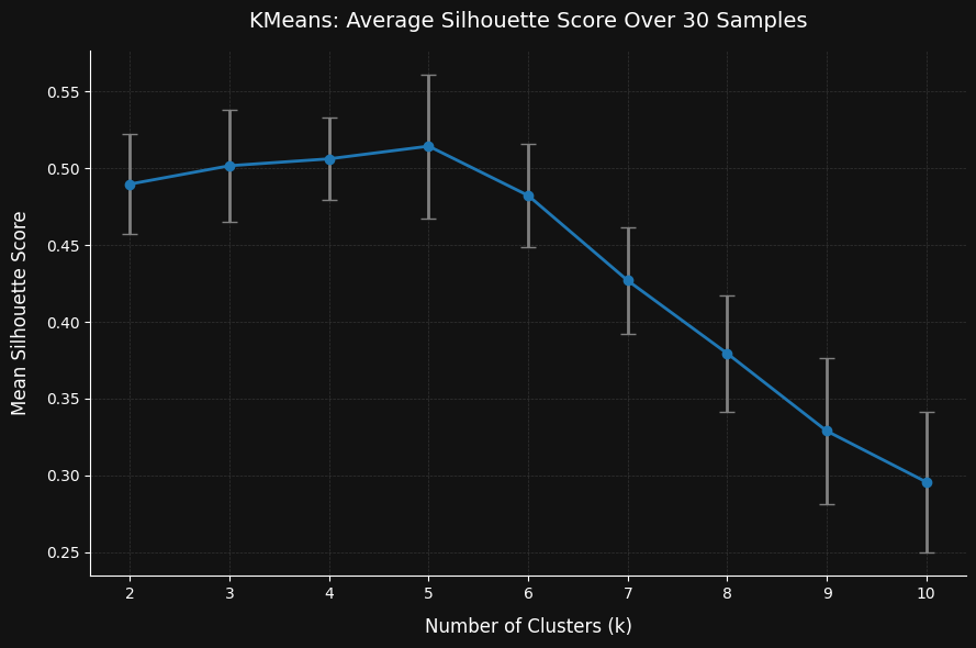
The plot above shows that after running 30 iterations on samples of just 50 records each (roughly 0.5% of the full dataset), the algorithm was still able to correctly identify the optimal number of clusters. Interestingly, the silhouette score consistently peaked at the true number of clusters, and began to decline beyond that point.

One notable observation is that the method seems to lean toward underestimating the number of clusters rather than overestimating it. This makes intuitive sense: when using small samples, there’s a higher chance of missing smaller or less dense clusters, which can lead the algorithm to favor fewer clusters overall. It highlights an important tradeoff—sampling helps with scalability, but may reduce sensitivity to rare patterns if the sample size is too small.

Step 2: Sampling repeatedly to estimate centroid values

INPUT:
    - Dataset of samples
    - M: Number of clusters
    - R: Number of new clusters explored per sample
    - H: Number of closest clusters retained
    - sample_number: Number of random sample batches
    - sample_size: Number of data points per batch
    - convergence_tol: Stopping threshold for centroid change

INITIALIZE:
    - Take initial sample of size `sample_size`
    - Randomly select M points as initial centroids
    - Initialize cluster similarity matrix S to zeros
    - Set iteration counter to 0

FOR each sample_iter in 1 to sample_number:
    - Draw a new random sample of `sample_size` points
    - Compute Euclidean distance from each point to each centroid
    - For each point, randomly assign H clusters from M as its initial neighborhood K(n)

    FOR each iteration up to 100:
        - Increment global iteration counter
        - Initialize empty cluster assignment lists and new similarity matrix S_new

        FOR each point n in the sample:
            - Find the closest cluster c_bar in its current neighborhood K(n)
            - Compute transition probability p(c | c_bar) from similarity matrix S
            - Sample R new candidate clusters based on p
            - Merge candidates with current neighborhood
            - Compute distances to all clusters in the merged set
            - Keep H closest clusters as new K(n)
            - Record assignments and update S_new accordingly

        - For each cluster c:
            - If it has assigned points:
                - Find the medoid (point with smallest total distance to others)
                - Update new centroid value for cluster c

        - Check centroid shift. If below tolerance, break loop
        - Update centroid values using weighted average over all iterations
        - Replace S with S_new

OUTPUT:
    - Final centroid values (shape M × D)

What This Algorithm Does:

This is a sampling-based clustering algorithm that tries to find good centroids (cluster centers) by repeatedly working on small batches of data rather than the full dataset. It uses a truncated EM-like approach that refines which clusters each data point is closest to, without exhaustively comparing it to all clusters every time.

Step-by-Step Explanation:

1. Initial Sampling & Centroid Guess
   • You randomly take a small batch of data (e.g. 50 samples).
   • From this batch, you pick M random points to act as the initial centroids.
2. Repeated Sampling Loop (Outer Loop)
   • You repeat this process multiple times (sample_number).
   • In each loop, a new random batch of data is selected from the full dataset.
3. Truncated Clustering (Inner Loop)
   • For each point in the batch, you only consider a small set of potential clusters (starting with a random subset).
   • The point is assigned to the closest cluster from that small set.
4. Neighborhood Expansion
   • Based on this closest cluster, the algorithm looks at transition probabilities (how frequently points moved from one cluster to another in the past).
   • It uses this to sample new potential clusters to consider, adding them to the point’s neighborhood.
5. Refinement Step
   • From the expanded neighborhood, the point chooses the closest cluster(s) again and updates its assignment.
   • This is repeated for multiple iterations until the centroids stop changing significantly.
6. Centroid Update
   • For each cluster, the most representative point (medoid) is chosen—this is the point in the cluster with the smallest total distance to all others.
   • These new centroids are averaged with the previous centroids, weighted by how many times the loop has run, so that centroids evolve smoothly.
7. Repeat Until Done
   • You do this for multiple batches of data, refining the centroids over time.

What You Get in the End:

• A set of M centroids that represent clusters found efficiently by sampling and refinement, not by comparing every point to every cluster.
• These centroids can then be used to assign cluster labels to new data points.

Actual Python code is found below:

from sklearn.metrics import pairwise_distances
import numpy as np

# === Config ===
M = 5  # Total number of clusters (centroids)
R = 5  # Number of new clusters explored
H = 1  # Number of closest clusters retained

sample_number = 5
sample_size = 50
convergence_tol = 1e-4

# === Step 1: Initialize centroids from the first batch ===
X_df = dummy_data.sample(n=sample_size, random_state=1000)
X = X_df.values
N, D = X.shape

mu_indices = np.random.choice(N, M, replace=False)
S = np.zeros((M, M))
centroid_values = X[mu_indices]

current_iteration =0
# === Iterate over random samples ===
for sample_iter in range(sample_number):
    print(f"Sample {sample_iter + 1}/{sample_number}", end='\r')
    X_df = dummy_data.sample(n=sample_size, random_state=1020 + sample_iter)
    X = X_df.values
    N, D = X.shape

    dist_X_to_centroids = pairwise_distances(X, centroid_values, metric='euclidean')  # shape (N, M)

    K = [set(np.random.choice(M, H, replace=False)) for _ in range(N)]
    for iteration in range(100):
        current_iteration+=1
        cluster_assignments = [[] for _ in range(M)]
        S_new = np.zeros((M, M))

        for n in range(N):
            k_n = list(K[n])
            x_n = X[n]
            distances = [dist_X_to_centroids[n, c] for c in k_n]
            c_bar_idx = np.argmin(distances)
            c_bar = k_n[c_bar_idx]

            if S[c_bar].sum() == 0:
                p = np.ones(M) / M
            else:
                p = S[c_bar] / S[c_bar].sum()

            nonzero_indices = np.flatnonzero(p)
            if len(nonzero_indices) < R:
                new_candidates = set(np.random.choice(M, size=R, replace=False))
            else:
                new_candidates = set(np.random.choice(M, size=R, p=p, replace=False))

            new_candidates = new_candidates - K[n]
            K_bar = K[n].union(new_candidates)

            dists = {c: dist_X_to_centroids[n, c] for c in K_bar}
            closest = sorted(dists, key=dists.get)[:H]
            K[n] = set(closest)

            for c in K[n]:
                cluster_assignments[c].append(n)
                S_new[c_bar, c] += 1

        new_centroid_values = []
        for c in range(M):
            members = cluster_assignments[c]
            if not members:
                new_centroid_values.append(centroid_values[c])
                continue

            intra_dists = pairwise_distances(X[members], X[members])
            intra_sums = np.sum(intra_dists, axis=1)
            new_center_idx = members[np.argmin(intra_sums)]
            new_centroid_values.append(X[new_center_idx])

        new_centroid_values = np.vstack(new_centroid_values)
        change = np.linalg.norm(centroid_values - new_centroid_values)
        if change < convergence_tol:
            break

        centroid_values = (new_centroid_values + ((current_iteration - 1) * centroid_values)) / current_iteration
        S = S_new

# Final output
print("\nFinal centroid values:", centroid_values)

Step 3: Using the final centroid features to classify unseen data

from sklearn.metrics import pairwise_distances
import numpy as np

def predict_cluster(X_new, centroid_values):
    """
    Assigns each sample in X_new to the nearest cluster centroid using Euclidean distance.

    Parameters:
        X_new: ndarray of shape (n_samples_new, D)
        centroid_values: ndarray of shape (M, D) – actual centroid feature vectors

    Returns:
        cluster_labels: ndarray of shape (n_samples_new,)
    """
    dists = pairwise_distances(X_new, centroid_values, metric='euclidean')
    cluster_labels = np.argmin(dists, axis=1)
    return cluster_labels

The prediction function (defined earlier) takes the centroid values obtained from the sampling-based clustering and assigns each new data point to the nearest centroid using a chosen distance metric. This effectively labels the new data according to the most similar cluster.

One key advantage of this approach is that the centroid values themselves act as the model parameters, offering an interpretable summary of each cluster. These centroids represent the most typical or central data points in each group, helping to characterize what kind of data belongs to which cluster.

Additionally, the method is flexible with respect to the distance metric. While Euclidean distance is commonly used, the implementation can be easily adapted to support other similarity or dissimilarity measures, such as mutual information, enabling more nuanced clustering in cases where non-linear relationships exist.

Evaluating Cluster Quality with Adjusted Rand Index

from sklearn.cluster import AgglomerativeClustering
from sklearn.metrics import adjusted_rand_score, pairwise_distances

# Get predicted labels using the final centroids
dgm_labels = predict_cluster(dummy_data.values, centroid_values)

# Compute full pairwise distance matrix (Euclidean)
dummy_data_dist_matrix = pairwise_distances(dummy_data.values, metric='euclidean')

# Run Agglomerative clustering on the entire dataset
agg_model = AgglomerativeClustering(n_clusters=3, metric='precomputed', linkage='average')
agg_labels = agg_model.fit_predict(dummy_data_dist_matrix)

# Compare the two clusterings
print("Adjusted Rand Index (D-GMM vs Agglomerative):", 
      adjusted_rand_score(dgm_labels, agg_labels))

To evaluate the effectiveness of the sampling-based clustering method, the results are compared against those produced by a standard Agglomerative Clustering algorithm applied to the full dataset. Agglomerative Clustering is a hierarchical approach that considers all pairwise distances and is often treated as a strong baseline due to its comprehensive nature.

The comparison is made using the Adjusted Rand Index (ARI), a metric specifically designed to assess the similarity between two clusterings:

• ARI evaluates whether pairs of points are clustered together or separately in both results.
• It corrects for chance groupings, making the score more robust and interpretable.
• Importantly, ARI is invariant to label permutations, meaning that it recognizes identical groupings even if the cluster label numbers differ between methods.

In this experiment, the Adjusted Rand Index between the sampling-based clustering and Agglomerative Clustering is:

Adjusted Rand Index (D-GMM vs Agglomerative): 0.7692

This score indicates a high degree of similarity, suggesting that the sampled approach is capable of approximating the results of full-data clustering with far fewer computations.

The sampling-based method used the following hyperparameters:

• M = 5: The total number of centroids (clusters) being learned.
• R = 5: The number of candidate clusters explored for each point in each iteration.
• H = 1: The number of closest clusters retained per point—representing a hard cluster assignment.

Overall, this result demonstrates that the truncated, sampling-based strategy can yield competitive clustering performance while being more computationally efficient than full pairwise methods.