Backtesting Financial Time Series Forecasting

Time series forecasting plays a critical role in decision-making across industries. However, creating a predictive model is not enough — assessing whether the model generalizes to future data is essential. This is where model assessment and backtesting come in. A poorly executed backtest can lead to inflated expectations, poor real-world performance, and wasted resources.

This article presents a principled approach to time series backtesting, with emphasis on stationarity, resampling techniques, and avoiding common biases. It also includes a decision framework for selecting the appropriate validation strategy based on model complexity and data constraints.

The Importance of Stationarity in Forecasting

A stationary time series is one whose statistical properties—such as mean, variance, and autocorrelation—are constant over time. In practical terms, a stationary series does not exhibit long-term trends or seasonality. Many classical models, including ARIMA and its variants, assume stationarity to ensure stable parameter estimates and meaningful forecasts. More contemporary models would usually also require stationary time series because it ensures that the learned patterns remain consistent over time and do not reflect temporary trends or structural shifts that may not persist in the future.

In deep learning and other non-linear models, while strict statistical stationarity is not always assumed in the same way as in traditional models (e.g., ARIMA), the presence of strong non-stationarity—such as changing means, variances, or dependencies—can still:

• Lead to unstable training and poor generalization
• Bias model performance toward recent behavior
• Increase the risk of overfitting to transient dynamics

Thus, even for architectures like recurrent neural networks (RNNs), temporal convolutional networks (TCNs), or transformers, normalizing, differencing, or stabilizing the data often significantly improves forecasting quality and model robustness.

Testing for Stationarity

The Augmented Dickey-Fuller (ADF) test is one of the most commonly used methods for detecting non-stationarity. It tests the null hypothesis that a unit root is present in the time series.

• Null hypothesis (H₀): The series is non-stationary (has a unit root).
• Alternative hypothesis (H₁): The series is stationary.

If the test statistic is significantly negative (beyond a critical threshold), the null hypothesis is rejected, indicating that the time series can be considered stationary. Conducting such tests prior to modeling is essential; otherwise, model results may be based on structural changes or trends that are unlikely to repeat in future data. If a time series is non-stationary, preprocessing might be required. Consider applying fractional differencing .

Backtesting and Model Assessment

In time series modeling, the goal is to estimate the true generalization error of a model — that is, how well it performs on future, unseen data. Since this cannot be observed directly, we rely on resampling strategies to approximate it.

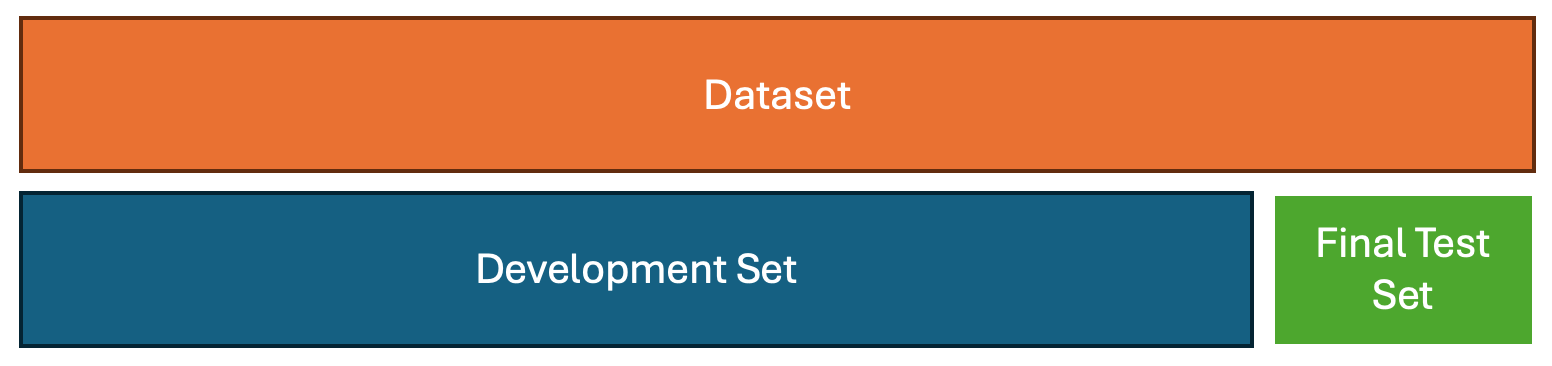
To ensure a rigorous and credible model evaluation process, the dataset should be divided into two distinct components: a development set and a final test set. The development set encompasses all data used during model construction, including training, validation, and backtesting. This is the portion of the data where model hypotheses are formed, parameters are tuned, and strategies are iteratively refined.

The final test set, by contrast, must remain completely untouched throughout the development process. It is to be used ideally only once, at the very end, to provide an unbiased estimate of the model’s real-world, out-of-sample performance. This final evaluation is typically conducted using a walk-forward test, which mirrors how the model would behave when deployed in production.

Crucially, the number of times the final test set is accessed should be recorded. Performance metrics such as the Sharpe ratio, commonly reported in financial contexts, can be artificially inflated if multiple evaluations are conducted on the same test data. To correct for this, appropriate statistical adjustments — such as Sharpe ratio deflation — should be applied to account for the risk of false positives due to multiple testing.

This strict separation is also designed to guard against a widespread and subtle pitfall: using backtesting as a research tool. When backtesting results are used to form hypotheses or drive model decisions, the evaluation becomes circular and unreliable. This practice leads to backtest overfitting — where the model performs well in historical simulation but fails under real-world conditions.1. 

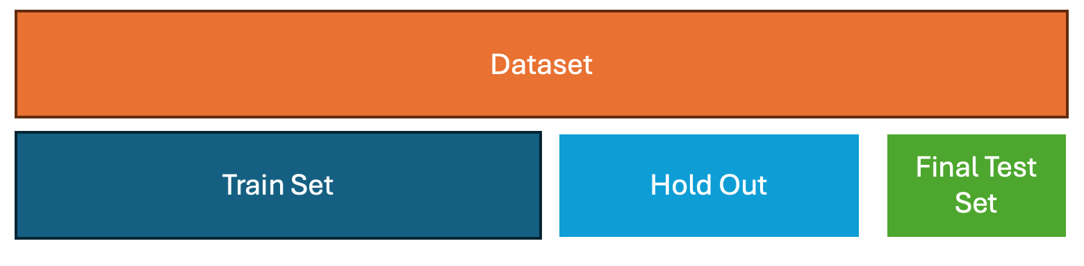
1 . Hold-Out Validation

How it works:

Split the dataset into two disjoint subsets:

• Training set: Used to train the model.
• Test set (hold-out): Used to evaluate performance.

For time series:

• The split must respect the time order.Example: Use data from 2015–2020 for training and 2021–2022 for testing.

Advantages:

• Simple to implement
• Computationally inexpensive

Limitations:

• High variance in performance estimate, especially with small datasets
• Result depends heavily on the specific split chosen

Use when: You have a large time series dataset and no hyperparameter tuning involved.

2. Cross-Validation (CV)

How it works:

Traditionally, k-fold CV splits the data into k equal parts (folds). The model is trained on k – 1 folds and validated on the remaining fold, repeated k times. The average performance is used as an estimate of generalization.

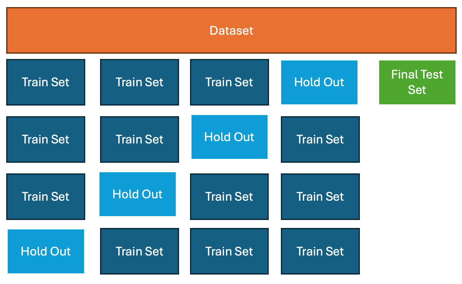
A variation of cross-validation tailored for time series data is anchored and non-anchored testing. The primary advantage of these approaches is that they preserve the chronological order of data and prevent data leakage, which is critical in time-dependent scenarios.

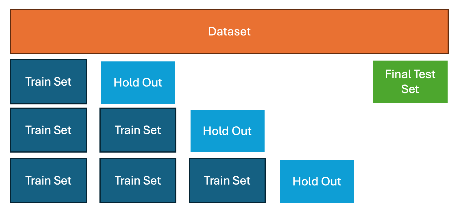
• In anchored testing (forward chaining), the training set grows with each iteration. For example:
  • Train on Period 1, test on Period 2
  • Train on Periods 1–2, test on Period 3
  • Train on Periods 1–3, test on Period 4, and so on.

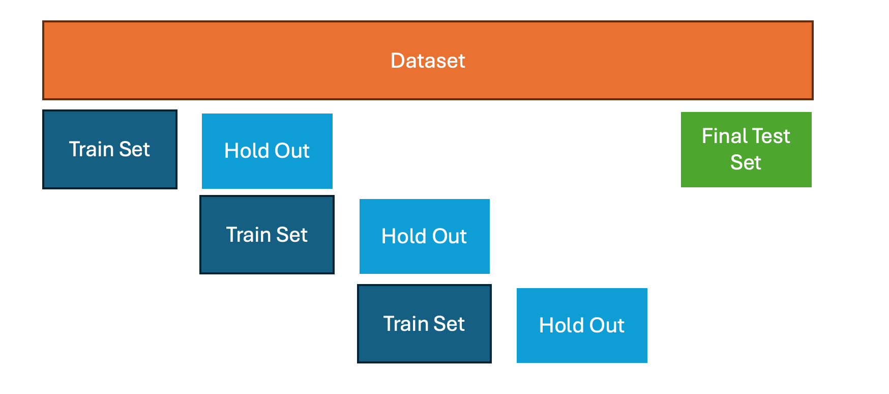
• In non-anchored testing (rolling origin), the training set slides forward without accumulating past data:
  • Train on Period 1, test on Period 2
  • Train on Period 2, test on Period 3
  • Train on Period 3, test on Period 4, etc..

Advantages:

• Reduces variance in error estimation
• More data-efficient than hold-out

Limitations:

• More computationally intensive
• Must be adapted for temporal order

Use when: You have moderate data and want a more reliable performance estimate than a single split.

3. Bootstrap

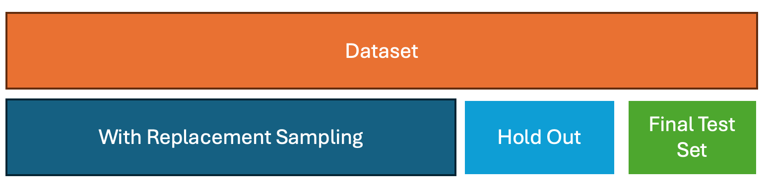
How it works:

Create multiple datasets by sampling with replacement from the original training data. The model is trained on each resampled dataset and tested on the out-of-bag observations (data not included in the sample).

In time series:

• Requires adaptation, such as moving block bootstrap or stationary bootstrap, to preserve autocorrelation
• The .632 or .632+ bootstrap adjusts for optimistic bias in performance estimates

Advantages:

• Effective with small datasets
• Provides uncertainty estimates (e.g., confidence intervals)

Limitations:

• May break time dependence if naively applied
• Less suitable for high-complexity models

Use when: You have a low-complexity model and limited data, and you need a reliable performance distribution.

4. Subsampling

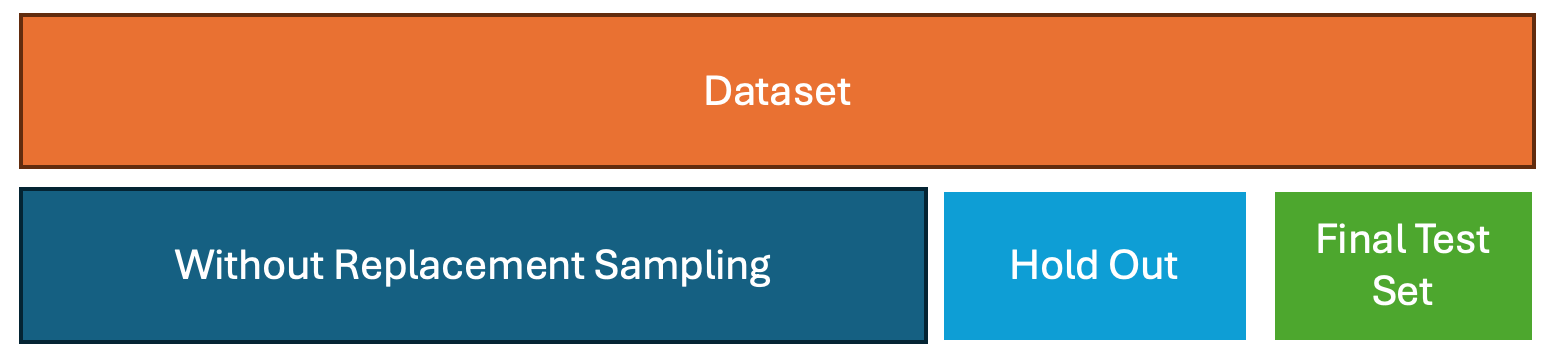
How it works:

Randomly draw subsets of the data without replacement to form training and validation sets. Repeated many times to estimate performance. Unlike bootstrap, each data point is used at most once in a sample.

In time series:

• Subsampling should be block-based to preserve temporal structure
• Allows you to test the model under multiple different temporal configurations

Advantages:

• Less bias than bootstrap in small samples
• Preserves more of the data’s temporal structure

Limitations:

• Still requires caution to avoid data leakage
• Fewer observations in each sample may increase variance

Use when: You need an alternative to bootstrap that avoids duplicate records, or want to reduce dependence on a single test set.

Key Pitfalls in Backtesting and Why They Matter

Backtesting can offer a false sense of security if methodological errors are not carefully avoided. Below are common pitfalls that undermine the reliability of backtest results, particularly in financial and economic forecasting.

Survivorship Bias

Using only the current universe of assets while ignoring companies that went bankrupt or were delisted skews performance metrics. This bias overestimates profitability by focusing only on surviving entities.

Look-Ahead Bias

Using information that was not publicly available at the time of a simulated trade introduces unrealistic advantages. Ensuring accurate timestamps and accounting for delays in data releases is critical.

Storytelling

Constructing post hoc narratives to justify observed patterns is a common cognitive trap. These explanations often lack statistical validity and obscure the true sources of performance.

Data Mining and Data Snooping

Fitting models on the testing set or conducting repeated backtests without proper control inflates the likelihood of overfitting. This leads to falsely optimistic evaluations of model accuracy.

Transaction Costs

Neglecting transaction costs results in inflated returns. Simulating realistic slippage, spreads, and execution delays is complex, but necessary for honest backtesting.

Outliers and Rare Events

Relying on a few extreme outcomes can misrepresent the typical performance of a strategy. These events may not recur and should be treated with appropriate statistical caution.

Shorting Constraints

Shorting assets requires borrowing, which depends on availability, cost, and market relationships. These factors are often unknown in backtests, leading to unrealistic assumptions about trade execution.

Conclusion

Effective time series forecasting goes beyond model building — it demands rigorous model assessment and backtestingto ensure reliable real-world performance. By incorporating principles like stationarity, choosing appropriate resampling techniques, and maintaining strict data integrity, practitioners can avoid common pitfalls such as data leakage, overfitting, and biases like survivorship or look-ahead bias.

This article has outlined a structured approach to validation — from simple hold-out methods to more advanced strategies like anchored cross-validation, bootstrap, and subsampling — each suited to different data scenarios and model complexities. By understanding when and how to use each method, forecasters can make better decisions, avoid misleading results, and ultimately deploy models that stand the test of time and changing data dynamics.